
Written by: Faizy Ahsan
Introduction
In the previous article in this series, we explained the use of transformer models to address the grammatical error correction (GEC) problem. Although transformer models have had remarkable success in this area, their large memory footprint and inference latency inhibit the widespread implementation of transformer-based automated GEC applications. In this article, we discuss compression techniques used to reduce model size and improve inference speed in production. Specifically, we present results from two model compression techniques: (1) distillation and (2) pruning. Our results show that model compression techniques improve inference speed but at the expense of output quality. The codes used in this study are available from our GitHub repository (https://github.com/scribendi/Pruning).
First, we describe the GECToR model (Omelianchuk et al. 2020), which uses only the transformer encoder portion (and not the decoder portion) to correct a given sentence. We then explain distillation and pruning techniques before presenting our results. Finally, we compare both techniques based on various evaluation metrics, including precision, recall, F0.5 score, model size, and inference speed. We then conclude with possible avenues for future research.
GECToR
Omelianchuk et al. (2020) developed a model called GECToR that demonstrated remarkable performance on the Conference on Computational Natural Language Learning (CoNLL) 2014 (Ng et al. 2014; F0.5 = 0.66) and the Building Educational Applications (BEA) (Bryant et al. 2019) (F0.5 = 0.73) test datasets. It produced inference speeds 10 times faster than comparative transformer-based sequence-to-sequence GEC models. As such, GECToR was used as a base model in our distillation and pruning experiments.
To train a GECToR model, training data is preprocessed so that each token in the source sentence is mapped to a tag with the help of the target sentence. The tags identify token transformations, which can be at a basic level, such as keep or delete, or g-transformations that involve more complex operations, such as the conversion of singular nouns into plurals. The default tag vocabulary size of a GECToR model is 5,000. Once the tagged training data is available, the transformer encoder layers of the GECToR model are trained to predict token tags for the given input sentences. The input sequences are then transformed based on their predicted tags. In testing mode, however, the test sentences are not preprocessed, and the source test sentences are fed directly into the trained GECToR model. The transformed source test sentences from the output of the trained GECToR model are subsequently evaluated against the target test sentences. The GECToR model approach is to use the transformer encoders as classifiers while completely avoiding the transformer decoder results, thereby increasing the inference speed.
Distillation
In distillation, or knowledge distillation (Hinton el al. 2015), a smaller architecture called Student Model is trained to mimic the output of a comparatively massive architecture called Teacher Model, as shown in Figure 1.
Let the Student Model be S, the Teacher Model be T, and their prediction scores be p(S) and p(T), respectively. The objective function of the distillation approach is then calculated as follows:

where the first part computes the loss of S on the labeled examples, L(p(S), p(T)) is a loss function (e.g., mean squared error) that computes the difference between p(S) and p(T), and a controls the magnitude of the second loss term.
Figure 1. Training data used to compute two losses (Teacher-Student and train data loss) and to optimize Student Model parameters.
The goal of learning in model distillation is to minimize Equation 1. As a result, the loss of S on the labeled examples is minimized, and the output of S will resemble the output of T for a given example. However, although applying a distillation technique results in a more compact model, the method can itself lead to computational overhead and decreased performance because two loss functions—the labeled loss and the student loss—must be minimized simultaneously (Turc et al. 2019; Sun et al. 2019).
Pruning
Pruning techniques remove a proportion of the model weights, yielding sparser models with lower memory requirements and comparable accuracy (LeCun et al. 1989; Hanson and Pratt 1988).
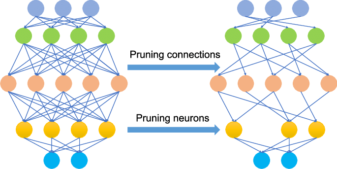
Figure 2. Pruning a neural network model (Sakkaf 2020).
Han et al. (2015) have determined the weights of a trained model to be pruned may be removed if their values fall below a certain threshold. The pruned model can then be retrained to achieve better accuracy. It is equally possible to use a set of thresholds so the model is pruned and retrained iteratively at each threshold (Gale et al. 2019; Lee et al. 2018; Molchanov et al. 2017). In their review of various pruning techniques, Blalock et al. (2020) proposed a benchmark for evaluating neural network pruning methods. Broadly, models can be pruned based on (1) structure (weights from different layers are pruned in unstructured pruning, while entire layers are pruned in structured pruning); (2) scoring (parameters are scored based on certain criteria, such as relevance and magnitude, either globally or locally, and are pruned accordingly); (3) scheduling (whereby the model is pruned at certain intervals); and (4) fine-tuning (the original weights before pruning are incorporated during the training of the pruned model).
Results
We evaluated the GECToR model using both distillation and pruning techniques with respect to (1) inference speed (number of words predicted per second); (2) model accuracy (precision, recall, and F0.5 scores); and (3) model size (measured in megabytes, MB). We first present the results of our distillation experiments, followed by the pruning results, and finally a comparison of the two techniques.
Results with Distillation
In Table 1, we show the results from two GECToR models on the CoNLL 2014 test set, which contains 1,312 sentences. One GECToR model with 12 BERT encoder layers and another with six cased DistilBERT layers were trained on a Scribendi dataset of approximately four million sentences. It should be noted that we used the cased version of DistilBERT rather than the uncased version, given that the input sentences can feature both cased and uncased words.
Table 1. GECToR with and without Distillation (CoNLL 2014 Test Set)
| Metrics | GECToR with 12 Bert Encoders | GECToR with Cased DistilBert Encoders | % Change with DistilBert (Cased) |
| Precision | 0.4423 | 0.4278 | -3.23 |
| Recall | 0.3951 | 0.3667 | -7.19 |
| F0.5 | 0.432 | 0.414 | -4.17 |
| Median words/sec | 3530.88 | 5563.76 | 57.57 |
| Model size | 417 MB | 252 MB | -39.57 |
We observe from Table 1 that the distillation technique increased the inference speed at the cost of some precision, recall, and F0.5. The distillation technique also reduced the memory required to store the trained models.
The following are selected examples of corrections from the two GECToR models for the CoNLL 2014 test set.
Example 1:
| Source Sentence | In a conclusion, there are both advantages and disadvantages of using social media in daily life. |
| Target Sentence | In conclusion, there are both advantages and disadvantages in using social media in daily life. |
| GECToR (12 BERT encoders) |
In conclusion, there are both advantages and disadvantages of using social media in daily life. |
| GECToR (six cased DistilBERT encoders) | In conclusionthere are both advantages and disadvantages of using social media in daily life. |
Example 2:
| Source Sentence | Some people spend a lot of time in it and forget their real life. |
| Target Sentence: | Some people spend a lot of time online and forget their real lives. |
| GECToR (12 BERT encoders) |
Some people spend a lot of time in it and forget their real lives. |
| GECToR (Six cased DistilBERT encoders) | Some people spend a lot of time in it and forget their real lives. |
Example 3:
| Source Sentence | Without their concern and support , we are hard to stay until this time. |
| Target Sentence: | Without their concern and support, it is hard to stay alive for long. |
| GECToR (12 BERT encoders) |
Without their concern and support, it would it would be hard to stay until this time. |
| GECToR (Six cased DistilBERT encoders) | Without their concern and support, we are hard to stay until this time. |
The above two GECToR models were then evaluated using the Scribendi test set (5,000 sentences), as shown in Table 2.
Table 2. GECToR with and without Distillation (Scribendi Test Set)
| Metrics | GECToR with 12 BERT Encoders | GECToR with Cased DistilBertEncoders | % Change with DistilBert (Cased) |
| Precision | 0.4025 | 0.3974 | -1.27 |
| Recall | 0.1512 | 0.1327 | -12.24 |
| F0.5 | 0.302 | 0.2841 | -5.93 |
| Median words/second | 3474.96 | 6366.32 | 83.21 |
| Model size | 417 MB | 252 MB | -39.57 |
We observe from Table 2 that the distillation technique increased inference speed by 83.21% for the Scribendi test set. Again, this came at a cost in terms of precision, recall, and F0.5. In this case, the impact on precision was much smaller, and the impact on recall was greater compared to the previous dataset. It is worth noting here that the model sizes are independent of the datasets.
Below are selected examples of corrections from the two GECToR models for the Scribendi test set:
Example 4:
| Source Sentence | The Marine Corps has been under siege by sister services since it was re-organized. |
| Target Sentence | The Marine Corps has been under siege by its sister services since it was re-organized. |
| GECToR (12 BERT encoders) |
The Marine Corps has been under siege by Sister Services since it was re-organized. |
| GECToR (Six cased DistilBERT encoders) | The Marine Corps has been under siege by sister services since it was re-organized. |
Example 5:
| Source Sentence | Mean age of hip arthroscopy patient group was 36.76 (23-62) years. |
| Target Sentence | The mean age of the hip arthroscopy patient group was 36.76 (23-62) years. |
| GECToR (12 BERT encoders) |
The mean age of the hip arthroscopy patient group was 36.76 (23-62) years. |
| GECToR (Six cased DistilBERT encoders) | The mean age of the hip arthroscopy patient group was 36.76 (23-62) years. |
Example 6:
| Source Sentence | The ankle jerk reflex was diminished to the right side than the left. |
| Target Sentence | The ankle jerk reflex was diminished more on the right side than the left. |
| GECToR (12 BERT encoders) |
The ankle jerk reflex was diminished to the right side than the left. |
| GECToR (Six cased DistilBERT encoders) | The ankle-jerk reflex was diminished to the right side than the left. |
Results with Pruning
The pruning technique applied here was based on Sajjad et al. (2020), who have experimented with removing encoding layers from a pre-trained BERT model in various orders before fine-tuning and evaluating them against general language understanding evaluation (GLUE) tasks.
Since Sajjad et al. (2020) demonstrated that removal from the top encoder layer led to optimal performance, we chose to apply a similar strategy in our pruning experiment. We removed the top n BERT encoder layers from the pre-trained GECToR model and re-trained the resulting pruned model on the Scribendi training dataset (approximately four million sentences).
Table 3. Performance of the Pruned GECToR Models
(CoNLL 2014 Test Set)
| # of BERT encoders | Precision | Recall | F0.5 | Size (MB) | Median words/second |
| 3 | 0.3728 | 0.2677 | 0.3457 | 173 | 8676.72 |
| 6 | 0.4066 | 0.3383 | 0.3908 | 254 | 5838.37 |
| 9 | 0.4366 | 0.3870 | 0.4257 | 336 | 4450.53 |
| 12 | 0.4423 | 0.3951 | 0.4320 | 417 | 3530.88 |
We compared the results of the pruning technique for the GECToR models with different numbers of BERT encoders, as shown in Table 3. We observed that removing the top n (12, 9, 6, and 3) BERT encoder layers from the pre-trained GECToR model and then re-training increased the inference speed and significantly decreased the model size in accordance with the increase in pruning, as seen in Figure 3. These results suggest that a model with a desired decrease in model size and increase in inference speed can be produced with this pruning technique with only some negative impact on accuracy (which nevertheless needs to be considered).
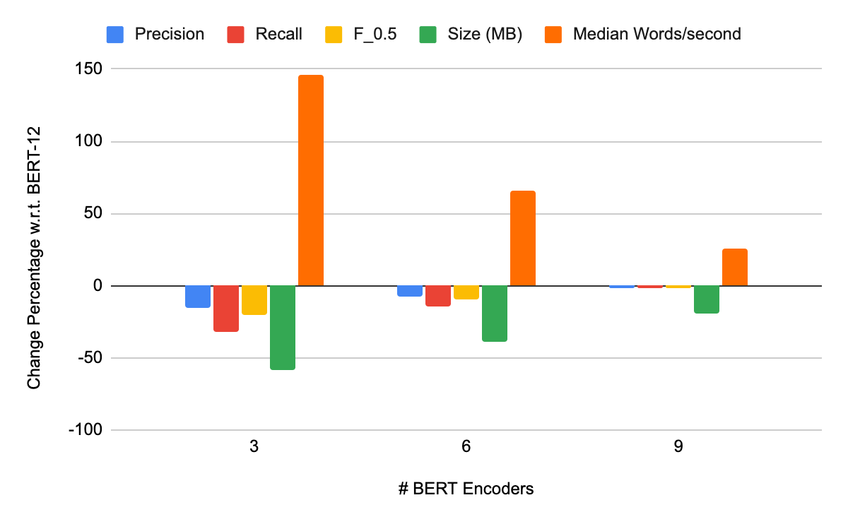
Figure 3. Comparison of evaluation metrics on the CoNLL-2014 test set for the GECToR models whose top n (9, 6, and 3) trained BERT encoder layers were removed and then retrained. BERT-12 is a GECToR model with 12 BERT encoders.
The following are selected examples of the corrections suggested by the GECToR model whose top six BERT encoder layers were removed after training and the pruned model after re-training.
Example 7:
| Source Sentence | In a conclusion, there are both advantages and disadvantages of using social media in daily life. |
| Target Sentence | In conclusion, there are both advantages and disadvantages in using social media in daily life. |
| GECToR (12 BERT encoders) |
In conclusion, there are both advantages and disadvantages of using social media in daily life. |
| GECToR (Six BERT encoders) |
In conclusionthere are both advantages and disadvantages of using social media in daily life. |
Example 8:
| Source Sentence | Some people spend a lot of time in it and forget their real life. |
| Target Sentence | Some people spend a lot of time online and forget their real lives. |
| GECToR (12 BERT encoders) |
Some people spend a lot of time in it and forget their real lives. |
| GECToR (Six BERT encoders) |
Some people spend a lot of time in it and forget their real life. |
Example 9:
| Source Sentence | Without their concern and support , we are hard to stay until this time. |
| Target Sentence | Without their concern and support, it is hard to stay alive for long. |
| GECToR (12 BERT encoders) |
Without their concern and support, it would it would be hard to stay until this time. |
| GECToR (Six BERT encoders) |
Without their concern and support, we are hard to stay until this time. |
We also followed the described pruning technique to evaluate the Scribendi test set; the results are shown in Table 4. Similar trends were observed (i.e., the inference speed increased at the cost of precision, recall and F0.5, as seen in Figure 4). Again, model sizes are independent of the datasets used.
Table 4. Performance of the Pruned GECToR Models
(Scribendi Test Set)
| # of BERT encoders | Precision | Recall | F0.5 | Size (MB) | Median words/second |
| 3 | 0.3618 | 0.0991 | 0.2364 | 173 | 9860.66 |
| 6 | 0.3883 | 0.1304 | 0.2783 | 254 | 6174.45 |
| 9 | 0.4001 | 0.1475 | 0.2980 | 336 | 4407.10 |
| 12 | 0.4025 | 0.1512 | 0.3020 | 417 | 3474.96 |

Figure 4. Comparison of evaluation metrics on the Scribendi test set for GECToR models whose top n (9, 6, and 3) trained BERT encoder layers were removed and then retrained. BERT-12 is a GECToR model with 12 BERT encoders.
Below are selected examples of the corrections suggested by the retrained GECToR model, whose top six Bert encoder layers were removed for the Scribendi test set.
Example 10:
| Source Sentence | The Marine Corps has been under siege by sister services since it was re-organized. |
| Target Sentence | The Marine Corps has been under siege by its sister services since it was re-organized. |
| GECToR (12 Bert encoders) |
The Marine Corps has been under siege by Sister Services since it was re-organized. |
| GECToR (Six Bert encoders) |
The Marine Corps has been under siege by sister services since it was re-organized. |
Example 11:
| Source Sentence | Mean age of hip arthroscopy patient group was 36.76 (23-62) years. |
| Target Sentence | The mean age of the hip arthroscopy patient group was 36.76 (23-62) years. |
| GECToR (12 Bert encoders) |
The mean age of the hip arthroscopy patient group was 36.76 (23-62) years. |
| GECToR (Six Bert encoders) |
The mean age of the hip arthroscopy patient group was 36.76 (23-62) years. |
Example 12:
| Source Sentence | The ankle jerk reflex was diminished to the right side than the left. |
| Target Sentence | The ankle jerk reflex was diminished more on the right side than the left. |
| GECToR (12 Bert encoders) |
The ankle jerk reflex was diminished to the right side than the left. |
| GECToR (Six Bert encoders) |
The ankle jerk reflex diminished to the right side of the left. |
Comparison of Distillation and Pruning Methods
We have presented results with one distillation and one pruning technique. In both, we observed an increase in inference speed at the cost of model accuracy, measured in terms of precision, recall, and F0.5 score. While we found that both techniques had similar impacts on these evaluation metrics, we argue that the pruning technique offers more options in terms of producing a compressed model with a desired increase in inference speed and an acceptable tradeoff in decreased accuracy. The comparison of distillation and pruning techniques is shown in Tables 5 and 6 as well as Figures 5 and 6.
Table 5. Comparison of Distillation and Pruning
(CoNLL 2014 Test Set)
| Precision | Recall | F0.5 | Size (MB) | Median words/second | |
| GECToR (Six cased DistilBERT encoders) | 0.4278 | 0.3667 | 0.4140 | 252 | 5563.76 |
| GECToR (Six BERT encoders) |
0.4066 | 0.3383 | 0.3908 | 254 | 5838.37 |
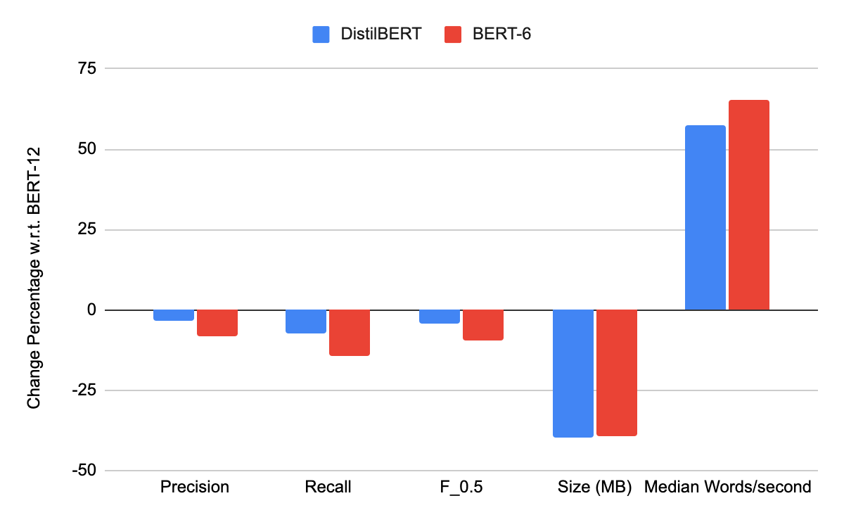
Figure 5. Comparison of distillation and pruning using the CoNLL 2014 test set. DistilBERT is a GECToR model with cased DistilBERT encoders. BERT-6 is a GECToR model trained with 12 BERT encoder layers before the top six BERT layers were removed, and the resulting model retrained. BERT-12 is a GECToR model with 12 BERT encoder layers.
Table 6. Comparison of Distillation and Pruning
(Scribendi Test Set)
| Precision | Recall | F0.5 | Size (MB) | Median words/second | |
| DistilBERT | 0.3974 | 0.1327 | 0.2841 | 252 | 6366.32 |
| BERT-6 | 0.3883 | 0.1304 | 0.2783 | 254 | 6174.45 |

Figure 6. Comparison of distillation and pruning using the Scribendi test set. DistilBERT is a GECToR model with cased DistilBERT encoders. BERT-6 is a GECToR model that was trained with 12 BERT encoder layers and then the top six BERT layers were removed, and the resulting model was retrained. BERT-12 was a GECToR model with 12 BERT encoder layers.
Conclusion
The goal of model compression is to yield a model for industrial application with faster inference speed and a smaller memory footprint without significant degradation in accuracy. In this article, we presented results for two model compression techniques: distillation and pruning. Our experiments demonstrated that both techniques resulted in decreased model size and increased inference speed. Although distillation was more effective in terms of model accuracy, pruning can provide a faster model. Moreover, the pruning method offers a greater range of control over inference speed, memory footprint, and accuracy. The results with pruning are encouraging when considering the industrial implementation of automated GEC tasks. Future research should explore further variations of pruning methods (such as those described in Blalock et al. 2020), as well as other model compression techniques, such as quantization (Asanović and Morgan 1991) and parameter sharing (Dehghani et al. 2018).
References
Asanović, Krste, and Nelson Morgan. 1991. “Experimental Determination of Precision Requirements for Back-Propagation Training of Artificial Neural Networks.” In Proceedings of the Second International Conference on Microelectronics for Neural Networks, 1991, 9–16. http://citeseerx.ist.psu.edu/viewdoc/summary?doi=10.1.1.38.2381.
Blalock, Davis, Jose Javier Gonzalez Ortiz, Jonathan Frankle, and John Guttag. 2020. “What is the State of Neural Network Pruning?” arXiv preprint arXiv:2003.03033.
Bryant, Christopher, Mariano Felice, Øistein E. Andersen, and Ted Briscoe. 2019. “The BEA-2019 Shared Task on Grammatical Error Correction.” In Proceedings of the Fourteenth Workshop on Innovative Use of NLP for Building Educational Applications, 2019, 52–75.
Dehghani, Mostafa, Stephan Gouws, Oriol Vinyals, Jakob Uszkoreit, and Łukasz Kaiser. 2018. “Universal Transformers.” arXiv preprint arXiv:1807.03819.
Gale, Trevor, Erich Elsen, and Sara Hooker. 2019. “The State of Sparsity in Deep Neural Networks.” arXiv preprint arXiv:1902.09574v1.
Han, Song, Huizi Mao, and William J. Dally. 2015. “Deep Compression: Compressing Deep Neural Networks with Pruning, Trained Quantization and Huffman Coding.” arXiv preprint arXiv:1510.00149.
Hanson, Stephen, and Lorien Pratt. 1988. “Comparing Biases for Minimal Network Construction with Back-Propagation.” Advances in Neural Information Processing Systems 1: 177–185.
Hinton, Geoffrey, Oriol Vinyals, and Jeff Dean. 2015. “Distilling the Knowledge in a Neural Network.” arXiv preprint arXiv:1503.02531.
LeCun, Yann, John S. Denker, and Sara A. Solla. 1989. “Optimal Brain Damage.” Advances in Neural Information Processing Systems 2: 598–605.
Lee, Namhoon, Thalaiyasingam Ajanthan, and Philip H. S. Torr. 2018. “Snip: Single-Shot Network Pruning Based on Connection Sensitivity.” arXiv preprint arXiv:1810.02340.
Molchanov, Dmitry, Arsenii Ashukha, and Dmitry Vetrov. 2017. “Variational Dropout Sparsifies Deep Neural Networks.” arXiv preprint arXiv:1701.05369.
Ng, Hwee Tou, Siew Mei Wu, Ted Briscoe, Christian Hadiwinoto, Raymond Hendy Susanto, and Christopher Bryant. 2014. “The CoNLL-2014 Shared Task on Grammatical Error Correction.” In Proceedings of the 18th Conference on Computational Natural Language Learning: Shared Task, 2014, 1–14.
Omelianchuk, Kostiantyn, Vitaliy Atrasevych, Artem Chernodub, and Oleksandr Skurzhanskyi. 2020. “GECToR—Grammatical Error Correction: Tag, Not Rewrite.” arXiv preprint arXiv:2005.12592.
Sajjad, Hassan, Fahim Dalvi, Nadir Durrani, and Preslav Nakov. 2020. “Poor Man’s BERT: Smaller and Faster Transformer Models.” arXiv preprint arXiv:2004.03844.
Sakkaf, Yaser. 2020. “An Overview of Pruning Neural Networks using PyTorch.” Medium. https://medium.com/@yasersakkaf123/pruning-neural-networks-using-pytorch-3bf03d16a76e.
Sun, Siqi, Yu Cheng, Zhe Gan, and Jingjing Liu. 2019. “Patient Knowledge Distillation for BERT Model Compression.” arXiv preprint arXiv:1908.09355.
Turc, Iulia, Ming-Wei Chang, Kenton Lee, and Kristina Toutanova. 2019. “Well-Read Students Learn Better: The Impact of Student Initialization on Knowledge Distillation.” arXiv preprint arXiv:1908.08962.
About the Author

Faizy Ahsan is a Ph.D. student in computer science at McGill University. He is passionate about formulating and solving data mining and machine learning problems to tackle real-world challenges. He loves outdoor activities and is a proud finisher of the Rock ‘n’ Roll Montreal Marathon.